The Structure of OLAP Cubes

The Structure of OLAP Cubes:

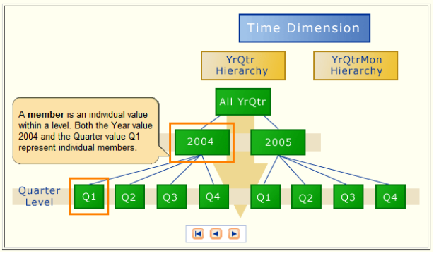
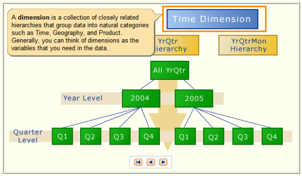
A cube is a set of data that is structured hierarchically. Unlike relational databases that use two-dimensional data structures (often in the form of columns and rows in a spreadsheet), cubes are logical, multidimensional models that consist of the following elements:
* one or more dimensions
* one or more levels
* one or more hierarchies
* members
If you’re not familiar with the structure and elements of OLAP cubes, you can go through the following series of pictures.

Understanding SAS Macro Symbol Tables

Rules for Creating and Updating SAS MacroVariables:
When the macro processor receives a request to create or update a macro variable during macro execution, the macro processor follows certain rules. Let’s look at those rules.

Suppose the macro processor receives a %LET statement during a macro call, as follows:
%let macvar=value;
The macro processor will take the following steps:
1. The macro processor checks to see whether the macro variable macvar already exists in the local symbol table. If so, the macro processor updates macvar in the local symbol table with the value value. If macvar does not exist in the local table, the macro processor goes on to step 2.
2. The macro processor checks to see whether the macro variable macvar already exists in the global symbol table. If so, the macro processor updates macvar in the global symbol table with the value value. If macvar does not exist in the global symbol table, the macro processor goes on to step 3.
3. The macro processor creates a macro variable named macvar in the local symbol table and assigns a value of value to it.

Similarly, suppose the macro processor receives the following reference during a macro call:
&macvar
The macro processor will take the following steps:
1. The macro processor checks to see whether the macro variable macvar exists in the local symbol table. If so, the macro processor retrieves the value of macvar from the local symbol table. If macvar does not exist in the local table, the macro processor goes on to step 2.
2. The macro processor checks to see whether the macro variable macvar exists in the global symbol table. If so, the macro processor retrieves the value of macvar from the global symbol table. If macvar does not exist in the global symbol table, the macro processor goes on to step 3.
3. The macro processor returns the tokens to the word scanner. A warning message is written to the SAS log to indicate that the reference was not resolved.

Remember that if the macro processor receives either a %LET statement or a macro variable reference (&macvar) in open code, it will check only the global symbol table for existence of the macro variable. If a macro program is not currently executing, a local symbol table does not currently exist.

SAS BI (OLAP Cube Studio): Tuning a SAS OLAP Cube

Watch the below video to learn how to tune your SAS OLAP Cube for better performance and accuracy!!
Happy Learning….

Audit Trail Datasets (to track modifications) in SAS

Definition of an Audit Trail:
The audit trail is an optional SAS file that you can create in order to log modifications to a SAS data file. Each time an observation is added, deleted, or updated, information is written to the audit trail about who made the modification, what was modified, and when.
Many businesses and organizations require an audit trail for security reasons. The audit trail maintains historical information about the data, which gives you the opportunity to develop usage statistics and patterns. The historical information enables you to track individual pieces of data from the moment they enter the data file to the time they leave.
The audit trail is also the only facility in SAS that stores observations from failed append operations and that were rejected by integrity constraints. The audit trail enables you to write a DATA step to extract the failed or rejected observations, use information describing why the observations failed to correct them, and then reapply the observations to the data file.

The audit trail is created by the default Base SAS engine and has the same libref and member name as the data file, but has a data set type of AUDIT. It replicates the variables in the data file and additionally stores two types of audit variables:
1) _AT*_ variables, which automatically store modification data
2) user variables, which are optional variables you can define to collect modification data

You initiate an audit trail in the DATASETS procedure with the AUDIT statement.

Eg:
/* Create SALES data set. */
data mylib.sales;
length product $9;
input product invoice renewal;
datalines;
FSP 1270.00 570
SAS 1650.00 850
STAT 570.00 0
STAT 970.82 600
OR 239.36 0
SAS 7478.71 1100
SAS 800.00 800
;
run;
/* Create an audit trail with a user variable. */
proc datasets lib=mylib nolist;
audit sales;
initiate;
user_var reason_code $ 20;
run;

The following example inserts an observation into MYLIB.SALES.DATA and prints the update data in the MYLIB.SALES.AUDIT.
/* Do an update. */
proc sql;
insert into mylib.sales
set product = ‘AUDIT’,
invoice = 2000,
renewal = 970,
reason_code = “Add new product”;
quit;
/* Print the audit trail. */
proc sql;
select * from mylib.sales(type=audit);
quit;

Updated Data in MYLIB.SALES.AUDIT Dataset:
The SAS System

product reason_code _ATOPCODE_ _ATUSERID_ _ATDATETIME_
________________________________________________________________________________
AUDIT Add new product DA xxxxxx 31OCT2007:11:24:32

Source: SAS Online Doc

Issue while ‘Redefining an Already Existing SAS Data Set Variable’

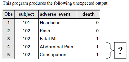
Often you want to redefine an already existing variable within a SAS DATA step. As simple as this may sound, it can lead to unexpected results if not done carefully. The following example displays some unexpected behavior that may occur when you redefine a variable within a DATA step. In this example you want to flag the subject who had the “Fatal MI” adverse event as having died (death = 1).

**** INPUT SAMPLE ADVERSE EVENT DATA WHERE SUBJECT = PATIENT ID
**** AND ADVERSE_EVENT = ADVERSE EVENT TEXT.;
data aes;
input @1 subject $3.
@5 adverse_event $15.;
datalines;
101 Headache
102 Rash
102 Fatal MI
102 Abdominal Pain
102 Constipation
;
run;
**** INPUT SAMPLE DEATH DATA WHERE SUBJECT = PATIENT NUMBER AND
**** DEATH = 1 IF PATIENT DIED, 0 IF NOT.;
data death;
input @1 subject $3.
@5 death 1.;
datalines;
101 0
102 0
;
run;
**** SET DEATH = 1 FOR PATIENTS WHO HAD ADVERSE EVENTS THAT
**** RESULTED IN DEATH.;
data aes;
merge death aes;
by subject;
if adverse_event = “Fatal MI” then
death = 1;
run;

Notice how the “Abdominal Pain” and “Constipation” observations also were flagged as death = 1. This happens because, by design, SAS automatically retains the values of all variables brought into a DATA step via the MERGE, SET, or UPDATE statement. In this example, because the “death” variable already exists in the “death” data set, that variable gets retained. When you assign death = 1 for “Fatal MI,” the subsequent records within that BY group are also set to 1. You should carefully read “Combining SAS Data Sets” in the Base SAS documentation for a thorough explanation of why this happens.

For the above example, the following code is a solution to the automatic variable retention feature.
**** FLAG EVENTS THAT RESULTED IN DEATH;
data aes;
merge death(rename = (death = _death)) aes;
by subject;
**** DROP OLD DEATH VARIABLE.;
drop _death;
**** CREATE NEW DEATH VARIABLE.;
if adverse_event = “Fatal MI” then
death = 1;
else
death = _death;
run;

Now you see that death = 1 only for the “Fatal MI” as desired. This was accomplished by changing the name of the “death” variable to “_death” on the way into the “aes” DATA step and then using the “_death” variable in defining a newly created “death” variable. Finally, “_death” is dropped from the outgoing copy of the “aes” data set.

Learning: Think twice before redefine a pre-existing variable within a DATA step.
Source : SAS® Programming in the Pharmaceutical Industry Book

Change-from-Baseline Calculation : Clinical SAS

Change-from-Baseline:
The purpose of using change-from-baseline analysis data sets is to measure what effect some therapeutic intervention had on some kind of diagnostic measure. A measure is taken before and after therapy, and a difference and sometimes a percentage difference are calculated for each post-baseline measure. These data sets are generally normalized vertical structure data sets. Here is an example of how such a data set could be created for systolic and diastolic blood pressure data.

data bp;
input subject $ week test $ value;
datalines;
101 0 DBP 160
101 0 SBP 90
101 1 DBP 140
101 1 SBP 87
101 2 DBP 130
101 2 SBP 85
101 3 DBP 120
101 3 SBP 80
202 0 DBP 141
202 0 SBP 75
202 1 DBP 161
202 1 SBP 80
202 2 DBP 171
202 2 SBP 85
202 3 DBP 181
202 3 SBP 90
;
run;

**** SORT DATA BY SUBJECT, TEST NAME, AND WEEK;
proc sort data = bp;
by subject test week;
run;
**** CALCULATE CHANGE FROM BASELINE SBP AND DBP VALUES.;
data bp;
set bp;
by subject test week;
**** CARRY FORWARD BASELINE RESULTS.;
retain baseline;
if first.test then baseline = .;
**** DETERMINE BASELINE OR CALCULATE CHANGES.;
if visit = 0 then baseline = value;
else if visit > 0 then
do;
change = value – baseline;
pct_chg = ((value – baseline) /baseline )*100;
end;
run;